Basics of Neural Networks

by Lekhya, on 3/11/2024

Deep learning is a subset of machine learning that imitates the intricate neural networks of the human brain, enabling computers to independently detect patterns and make decisions by analyzing large amounts of unstructured data. This technology powers applications such as facial recognition, natural language processing, and autonomous driving.

Artificial Neural Network (ANN)

ANN comprises of multiple layers of interconnected nodes called neurons that help in processing and learning from the input data.

A fully connected ANN has an input layer, several hidden layers, and an output layer. The input layer receives the input data and transmits it to the next layer, which is typically a hidden layer. As the input progresses through the layers of the ANN, it undergoes various non-linear transformations. Ultimately, the output layer generates the final output.

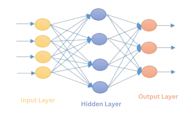
Neurons within an ANN are interconnected, and each connection is associated with a weight that determines the influence one neuron has on another. As data flows through the network, a weighted sum is computed, which enables the model to learn from the data. During training, these weights are adjusted to enhance the model's accuracy and performance.

Neural Network Architectures

Deep learning models excel at a variety of tasks due to their ability to automatically identify patterns and extract features from data. The most commonly utilized architectures include:

1. Feedforward Networks (FFNs): These networks exhibit a linear flow of data and are often employed in image processing and natural language processing tasks.
2. Convolutional Neural Networks: Primarily used for image and video analysis, CNNs are adept at object detection, image classification, and image segmentation.
3. Recurrent Neural Networks (RNNs): Designed for processing sequential data, RNNs are ideal for applications such as time series analysis and natural language processing.

Neural Network Layers

A neural network is structured with multiple layers, and its architecture influences the types of data it can process. Key types of neural network layers include:

1. Dense (Fully Connected) Layer: Each neuron in this layer connects to every neuron in the preceding layer, capturing global patterns within the data.
2. Convolutional Layer: Utilizes convolution operations to extract significant features from images.
3. Recurrent Layer: Incorporates feedback loops, providing context from previous steps, making them suitable for sequential data processing.
4. Pooling Layer: Reduces the spatial dimensions of the data, aiding in feature selection by retaining essential features while discarding less critical information.

Forward and Backward Propagation

Weights and Biases

In the training process of a neural network, weights and biases are crucial for optimizing performance. Weights are numerical values assigned to each connection between neurons, determining the strength of influence one neuron exerts over another. Weights are initialized to random in order to break symmetry. If all weights were initialized to the same value, each neuron would learn the same features during training, thus affecting the network's ability to learn complex patterns. Biases, in contrast, are typically initialized to zero. They shift the activation function and provide an additional parameter that allows the model to adapt flexibly to the data.

Forward Propagation

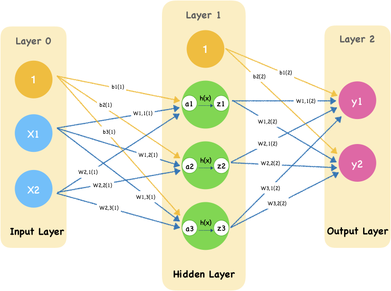
Forward propagation is the process through which input data is passed through the various neural network layers to produce an output. The steps are as follows:

1. Input Layer: The raw data is fed into the network through the input layer

2. Weighted Sum Calculation: Each neuron in the hidden layers computes a weighted sum using the input data and the weights associated with the connections. The input data is transformed as:

   $$z=W^{T}x+b=(w_{1,:},x_1+b_1,w_{2,:}{x}_2+b_2+...+w_{n,:}{x}_n+b_n{)}^T$$

   where $z$ is the network output, $w$ represents the weights, $x$ denotes the inputs, and $b$ is the bias.

3. Activation Function: The weighted sum is then transformed using an activation function, to determine the neuron's output, which is forwarded to the next layer

4. Output Layer: This process continues through all hidden layers until the output layer is reached, yielding the final prediction.

Backward Propagation

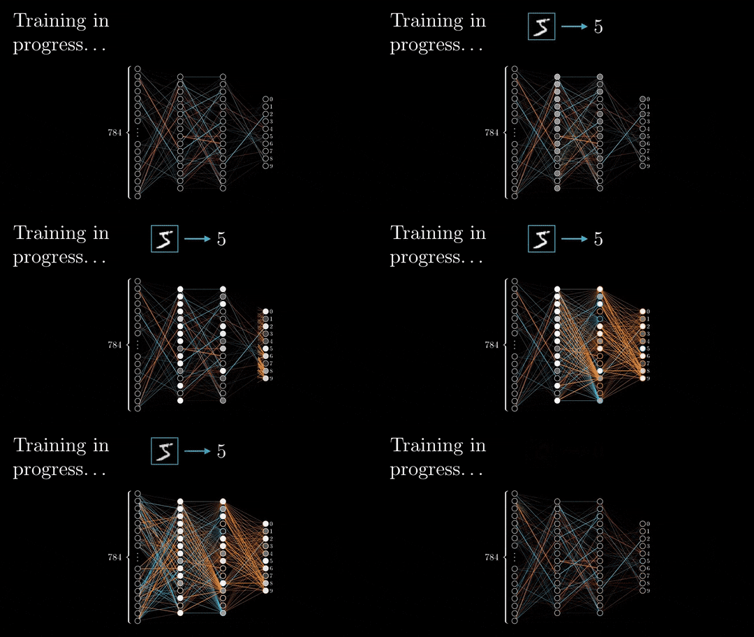
Backward propagation, or backpropagation, is the method employed to minimize loss by updating the weights and biases. The process consists of the following key steps:

1. Loss Calculation: After the forward pass, the difference/error between the predicted output and the actual output is calculated using a loss function. Common loss functions used are Mean Squared Error for regression tasks and Cross-Entropy Loss for classification tasks.
2. Gradient Calculation: The gradients of the loss function are calculated with respect to each weight and bias using the chain rule of calculus. This determines how changes in weights and biases impact the overall loss.
3. Weight Update: The calculated gradients are used to update the weights and biases, typically using optimization algorithms like Gradient Descent. This adjusts the parameters in the direction that minimizes the loss:$$w^{\prime }=w-\eta \cdot \frac{\partial \mathcal{L}}{\partial w}$$where $\eta$ represents the learning rate, and $\mathcal{L}$ is the loss.
4. Optimizers: Several optimization algorithms can be used to enhance the convergence process, such as:
   • Stochastic Gradient Descent (SGD): Updates weights using a random subset of data, improving computational efficiency for large datasets.
   • RMSprop: Builds on SGD by maintaining a moving average of squared gradients, which helps adjust the learning rate dynamically, especially effective in non-stationary environments.
   • Adam (Adaptive Moment Estimation): Combines the strengths of both RMSprop and SGD. By using first and second moments of gradients, Adam adapts learning rates for each parameter, making it robust and often more effective for diverse tasks.
5. Iteration: The forward and backward propagation steps are repeated for numerous iterations (epochs) until the model converges to an optimal set of weights that minimize the loss function.

Activation Functions

The input to a neural layer is derived from the previous layer as a weighted sum of its inputs, augmented by a bias term. Since this input can take any value from −∞ to +∞, activation functions are employed to transform this input before it progresses to the next layer. This transformation determines whether a neuron will be activated.

Types of Activation functions

1. Step Function

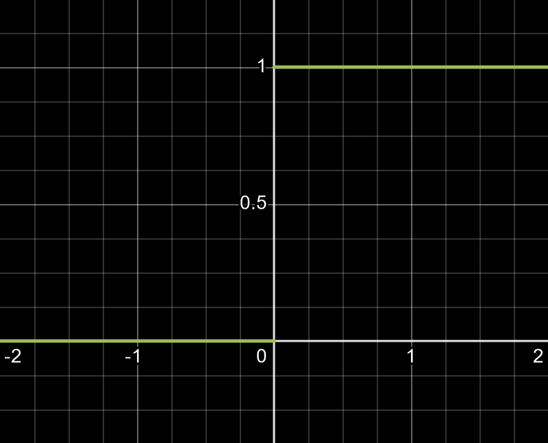
It is the most basic activation function. It activates a neuron if the net input exceeds a defined threshold. However, it lacks the flexibility to model more complex patterns, as it only outputs binary values (0 or 1), limiting the network's ability to learn nuanced relationships.

$$f(x)=\{\begin{array}{ll}1,& \text{if }x\ge 0\\ 0,& \text{if }x<0\end{array}$$

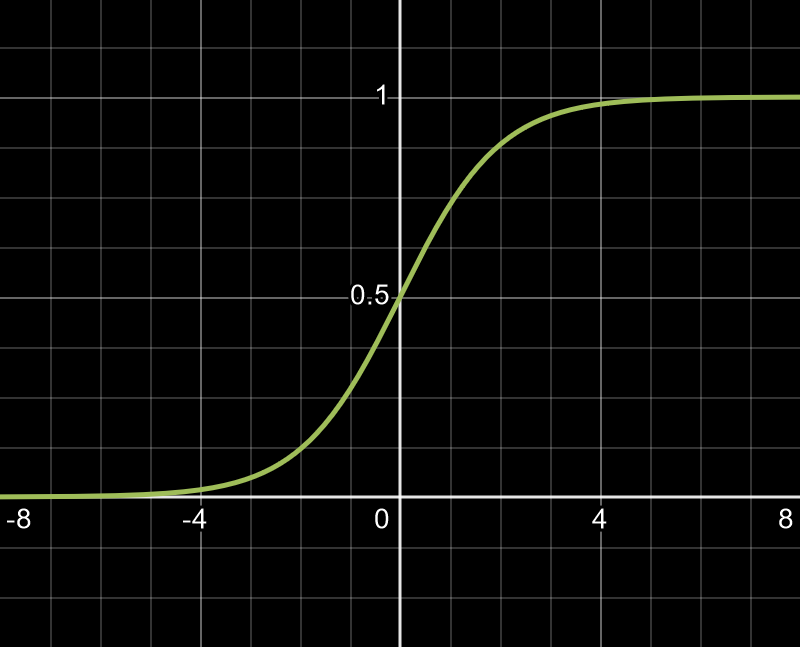
2. Sigmoid Function

Unlike the step function, the sigmoid function is continuous and differentiable, allowing smoother transitions between activated states. It introduces non-linearity, enabling the network to learn complex, layered patterns. However, it can suffer from vanishing gradients, especially in deep networks, limiting learning efficiency as layers increase.

$$\frac{1}{1+e^{-x}}$$

3. ReLU

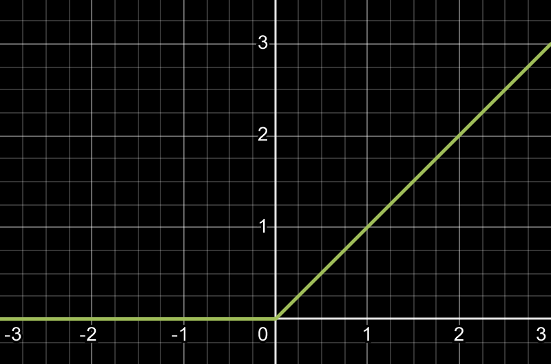
The Rectified Linear Unit (ReLU) is an activation function that improves neural network efficiency by allowing only positive inputs to activate neurons. If the input is negative, ReLU outputs zero, effectively keeping those neurons inactive. This sparsity helps the network focus on relevant features. Unlike sigmoid, ReLU mitigates the vanishing gradient problem, making it better suited for deep networks. However, ReLU can "die" if too many inputs are negative, causing neurons to stop learning.

$$f(x)=max(0,x)$$

4. Leaky ReLU

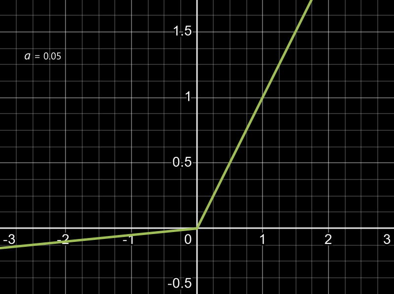
It is an enhanced version of ReLU function. If the input is negative, it is transformed to a small linear component of itself instead of 0. This enables the gradients to flow even for negative inputs, thus improving learning stability and reduces the risk of neurons becoming inactive.

$$f(x)=\{\begin{array}{ll}ax,& \text{if }x<0\\ x,& \text{otherwise}\end{array}$$

5. Tanh Function

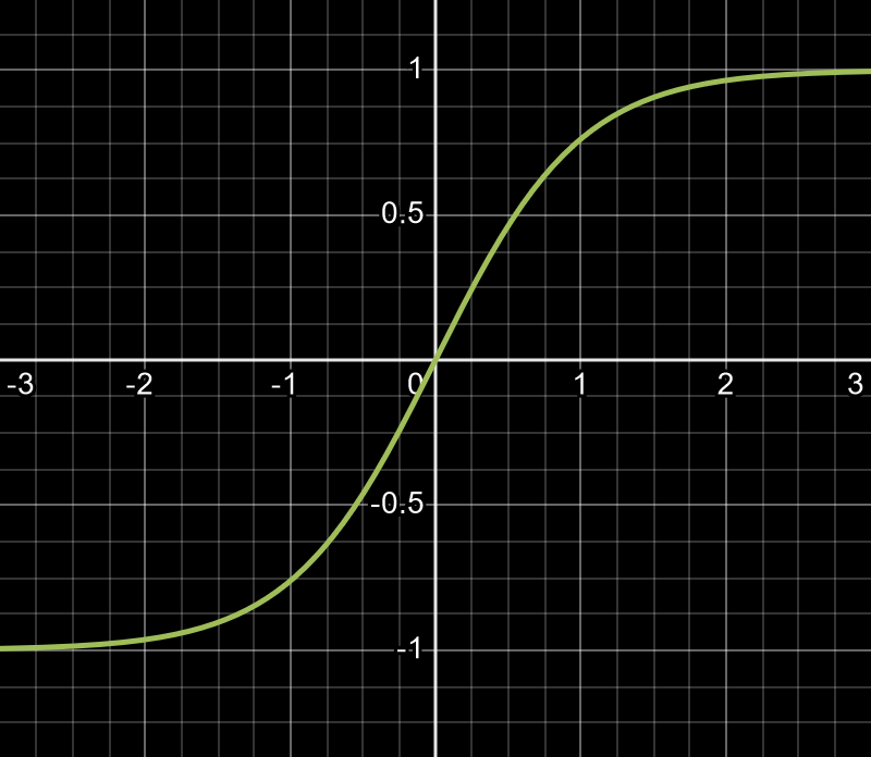
It is a non-linear function similar to sigmoid function but produces outputs in the the range -1 to +1. This range provides stronger gradients than sigmoid, improving training performance. However, like sigmoid, it can still experience vanishing gradients in deeper networks.

$$\tanh (x)=\frac{e^x-e^{-x}}{e^x+e^{-x}}$$

6. Softmax Function

It is a special activation function commonly used in the output layer of neural networks for multi-class classification problems. It converts the output into a probability distribution across multiple classes, assigning a probability score to each class. This helps to highlight the most likely prediction while reducing the influence of less likely classes, making Softmax ideal for final output layers in classification networks.

$$\text{softmax}(x_i)=\frac{e^{x_i}}{\sum _{j=1}^n{e}^{x_j}}$$

Conclusion

Deep neural networks are pivotal in advancing artificial intelligence, enabling the automatic learning of complex patterns from large datasets. This capability drives significant progress in areas like image recognition and natural language processing. With techniques such as backpropagation and innovative activation functions, these models adapt and excel across various applications. As a result, deep neural networks are reshaping AI and enhancing its influence across numerous industries.