Optimizers in Deep Learning

by Bhadra, on 24/03/2025

Optimizers are mathematical functions or algorithms which lower the loss function by updating the model’s learnable parameters (weights and biases) in response to the output of the loss function.

In order to maximize the efficiency of production by minimizing losses, to improve the training speed and to get the most accurate output, we need to know how to adjust the learning rates, weights and biases of the neural network during each training epoch. Optimizers help us in doing precisely this.

DIFFERENT TYPES OF OPTIMIZER

1. Gradient Descent
   1. Batch Gradient Descent(BGD)
   2. Stochastic Gradient Descent (SGD)
   3. Mini Batch Gradient Descent (MBGD)
2. Stochastic Gradient Descent with Momentum
   1. Mathematical representation:
   2. Disadvantages
3. Nesterov’s Accelerated Gradient
   1. Mathematical representation:
4. AdaGrad (Adaptive Gradient)
   1. Mathematical representation:
5. RMSProp (Root Mean Square Propagation)
   1. Mathematical representation:
6. Adam
   1. Mathematical representation:

Gradient Descent

Gradient Descent is an iterative optimization algorithm in which we approach the local minima by taking steps in the negative direction of the gradient at that point .

In Gradient Descent, we first compute the gradient (slope) of the loss function at a given point. Then, we update the parameters by moving in the opposite direction of the gradient, ensuring that we minimize the loss and move toward the optimal solution.

Batch Gradient Descent(BGD)

In BGD, the gradient of the function is calculated using the entire training dataset

$$W_{t+1}=W_t-\eta \cdot g_t$$

$W_{t+1}$ = Updated weight at step t+1

$W_t$ = Previous weight at step t

$\eta$ = Learning rate

$g_t$ = Gradient of the loss function at step t

Despite guaranteeing convergence, this method can be slow and prone to getting stuck in local minima when dealing with non-convex models.

Stochastic Gradient Descent (SGD)

SGD calculates the gradient of the cost function using only one randomly chosen data point in each iteration. It updates the model's parameters based on this individual gradient.

$$W_{t+1}=W_t-\eta \cdot g_t$$

Here,$g_t=\mathrm{\nabla }J(W_t,x_i,y_i)$ Gradient of the loss function for one sample $(x_i,y_i)$

This method updates the gradient frequently but can make the training process very noisy(many fluctuations)

Mini Batch Gradient Descent (MBGD)

MBGD is a compromise between BGD and SGD. It calculates the gradient of the cost function using a small batch of randomly chosen data points in each iteration. It updates the model's parameters based on this batch gradient.

$$W_{k+1}=W_k-\eta \cdot \left(\frac{1}{b}\right)\sum _{i=b}^b{g}_t$$$$b=\text{Mini-batch size}$$$$g_t=\mathrm{\nabla }J(W_k,x_i,y_i)=\text{for each sample in the batch}$$$$\text{The sum }\sum _{i=b}^b{g}_t=\text{averages the gradients over the mini-batch}$$

MBGD balances speed and stability, making it the most commonly used approach in deep learning.

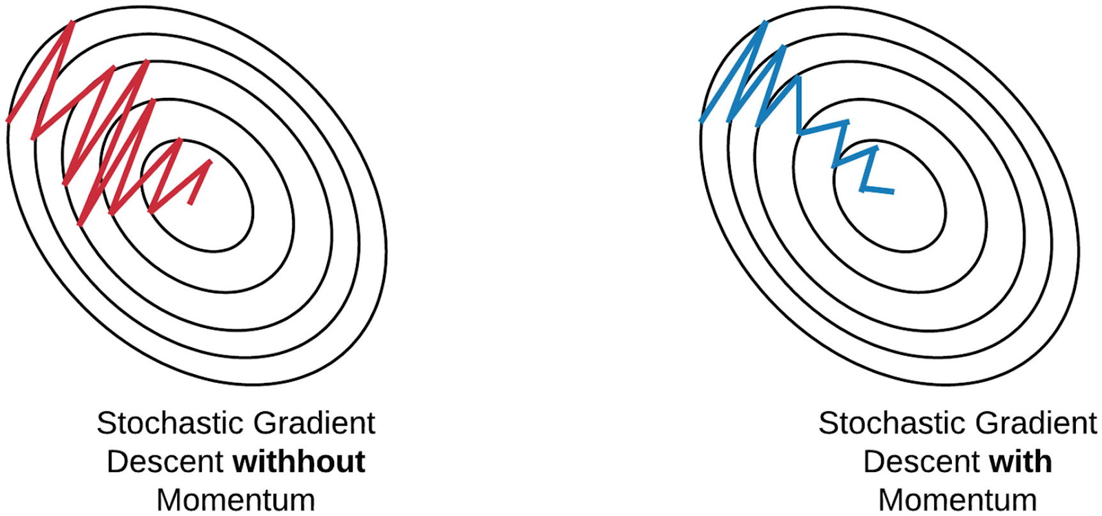
Stochastic Gradient Descent with Momentum

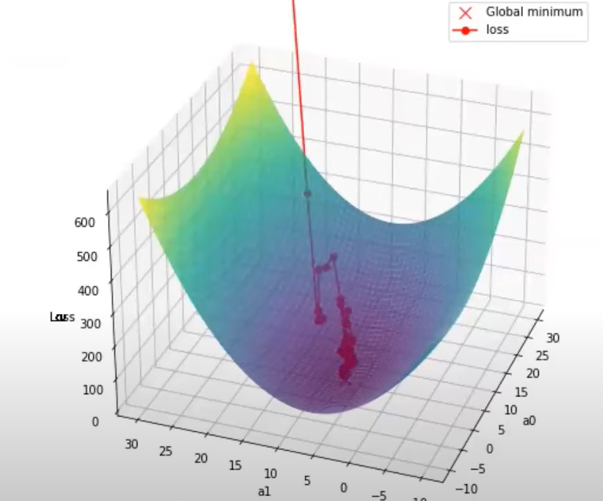
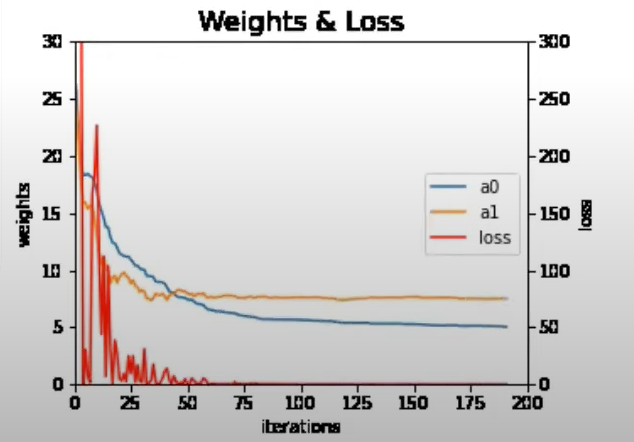
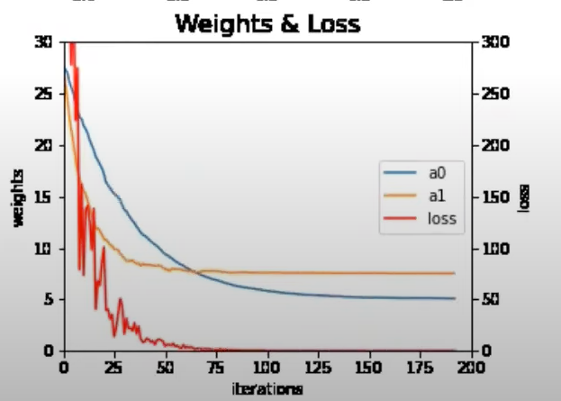
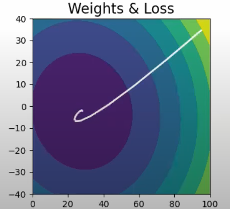
The path of learning in mini-batch gradient descent is zig-zag, and not straight. Thus, some time gets wasted in moving in a zig-zag direction. Momentum Optimizer in Deep Learning smooths out the zig-zag path and makes it much straighter, thus reducing the time taken to train the model.

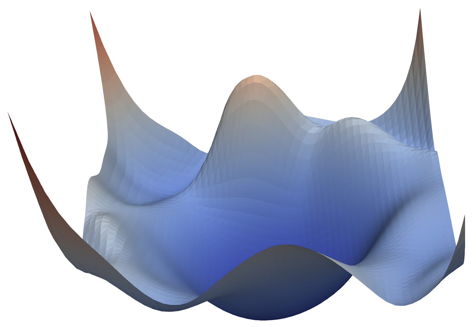
When faced with non-convex curves (i.e complex loss functions), the stochastic gradient descent posed multiple challenges;

• High curvature: small radius can lead to a higher curvature. Non-convex optimizations as shown in the figure usually have large curvature, which cannot be easily traversed using SGD methods

• Consistent gradients: When the change in slope of the curve decreases, especially in case of saddle point, the gradients become more consistent, leading to smaller updates and consequently more learning time.

• Noisy gradients: SGD usually follows a highly “noisy” (fluctuating) path which implies that it requires a more significant number of iterations to reach the optimal minimum.

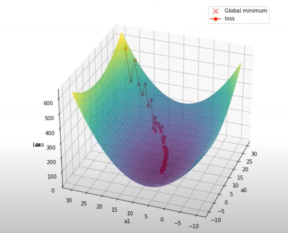
Momentum simulates the inertia of an object when it is moving, that is, by adding a fraction of the previous update to the current one, it retains the “velocity” (direction and speed) of the gradient descent.

Mathematical representation:

The change in the weights  is represented by:

$$W_{t+1}=W_t-V_t$$

Where,

• $V_t=\beta \cdot V_{t-1}+\eta \mathrm{\Delta }{W}_t$
• $V_t$: velocity of the gradient descent
• $\eta \mathrm{\Delta }{W}_t$: gradient of the loss
• $\beta$: momentum coefficient (usually between 0.5 and 0.99)
• $\beta \cdot V_{t-1}$: includes a fraction of the history of the velocities, helping it to utilise the past gradients.

The term $\beta$ is called a decay factor because it controls how much influence the previous velocity Vk−1 term has on the current velocity Vk.

Since βis typically chosen in the range $0\le \beta <1$, it gradually reduces the impact of past velocities over time. From the formula we see that, for calculating $V_t$ we have to calculate $V_{t-1}$ and for calculating $V_{t-1}$ we have to calculate $V_{t-2}$ and so on.

This way we are using the history of velocity to calculate the momentum. This part provides acceleration to the formula.

Disadvantages

• If the momentum value is set too high, it can cause the optimization process to overshoot the optimal solution,potentially leading to poor accuracy and oscillations around the minimum.

• The momentum value requires a critical hyperparameter that needs to be chosen manually and with precision  to pervent overfitting or overshooting.

Nesterov’s Accelerated Gradient

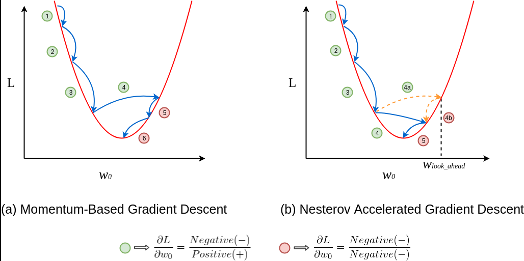
Nesterov’s Accelerated Gradient is a momentum based optimization technique that uses a "look ahead" method on the parameters to decide the gradient  in order to prevent overshooting.

In the traditional momentum method, the current gradient and the weighted sum of the past updates is calculated simultaneously and then a big jump or update is made using this accumulated gradient or "velocity" term as explained previously.

In contrast to this, Nesterov's method breaks down the process into two steps: First, NAG takes a "look ahead" step based on the weighted sum of the past updates (momentum term). Secondly, it calculates the gradient at this new "look ahead" point and makes a correction by adjusting the update based on this.

This breaking down of steps helps in preventing overshooting, allowing for more controlled updates.

Mathematical representation:

1. Calculating "look ahead term"

$$w_{\text{look-ahead}}=w-\beta \cdot v_{t-1}$$$$w:\text{ Current weights of the model.}$$$$v_{t-1}:\text{ Previous velocity term}$$

2. Calculating gradient

$$gradient=\mathrm{\nabla }f(w_{\text{look-ahead}})$$$$\text{Gradient is calculated at the new "look-out" position}$$

3. Updating the velocity term

$$v_t=\beta \cdot v_{t-1}+\eta \cdot gradient$$$$\eta :\text{ learning rate}$$$$\text{The new velocity is a combination of the previous velocities and the new gradient.}$$

4. Update the weights

$$w=w-v_t$$

AdaGrad (Adaptive Gradient)

In the previous optimization techniques, we saw that the learning rate was kept constant (at around 0.01). However, this can pose problems when we deal with datasets where the majority of the data is sparse and only some are dense.

In order to solve this problem, AdaGrad uses different learning rates for different parameters.

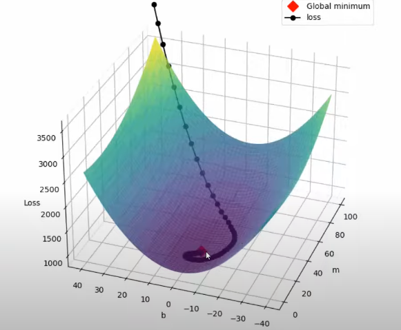
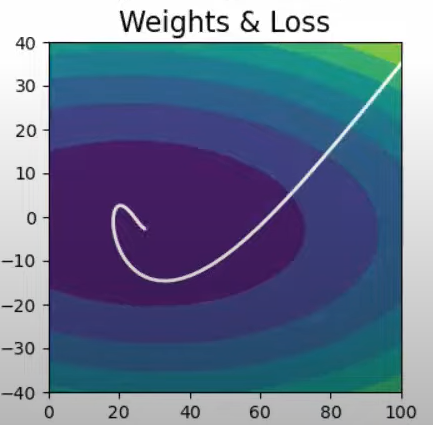
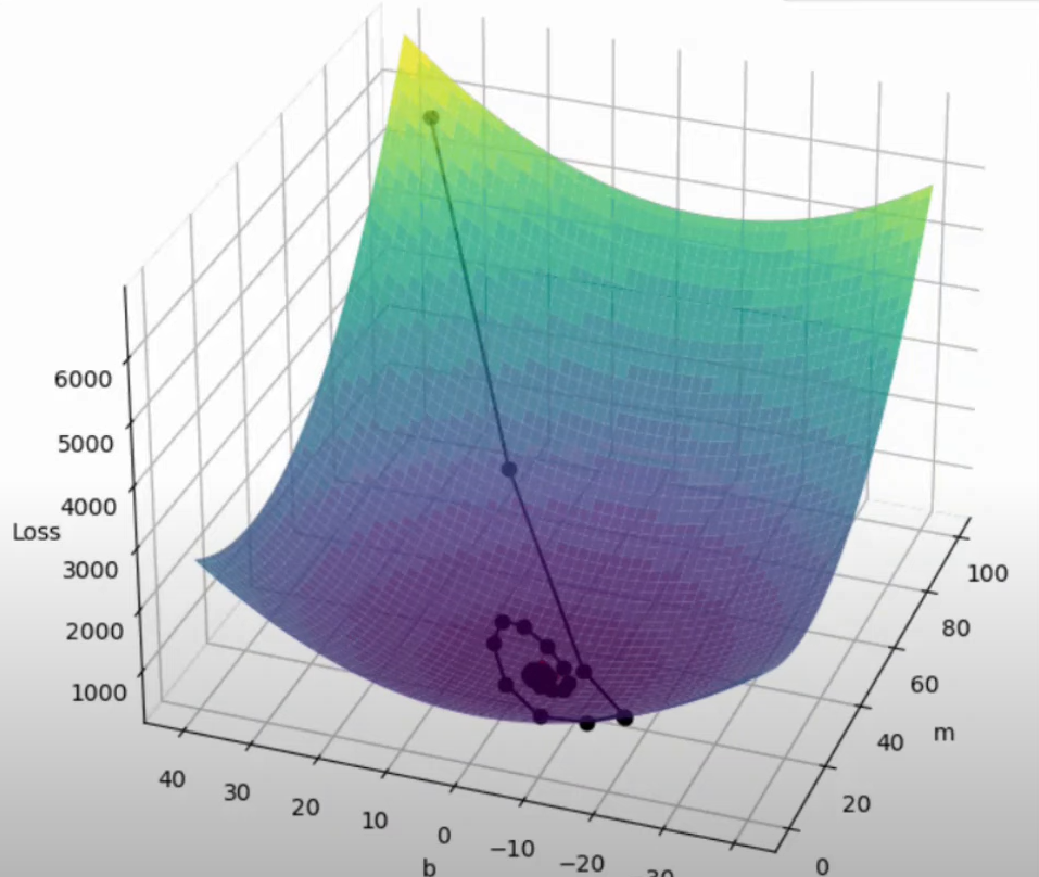
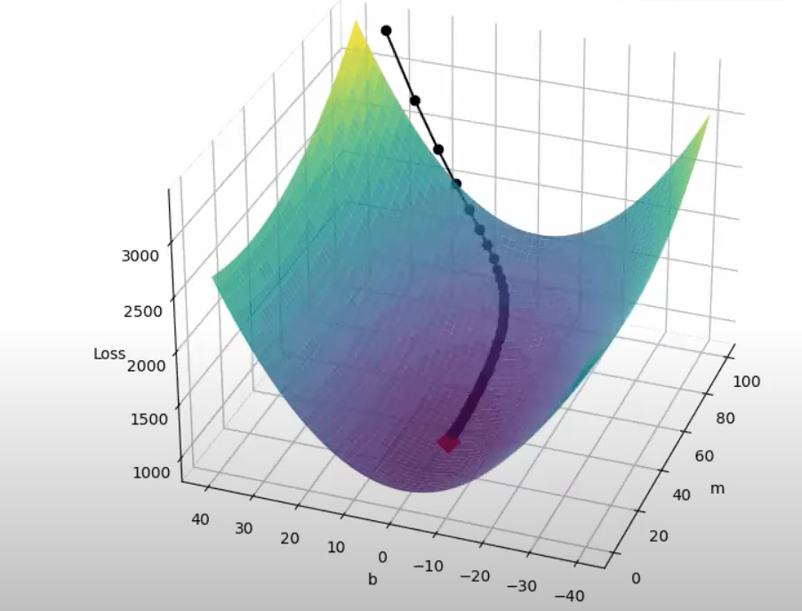
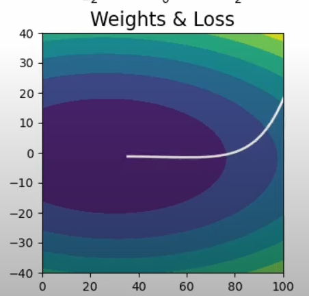
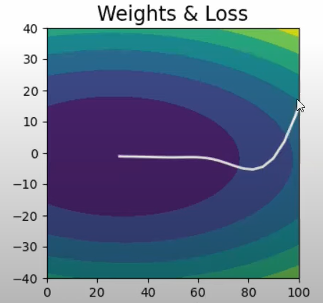
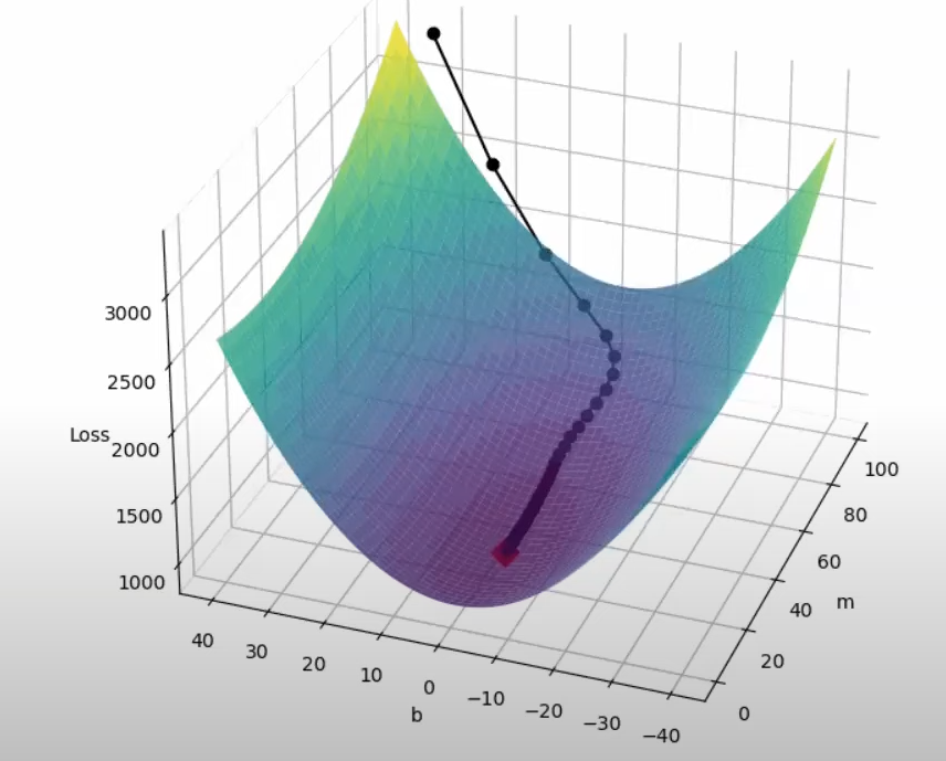
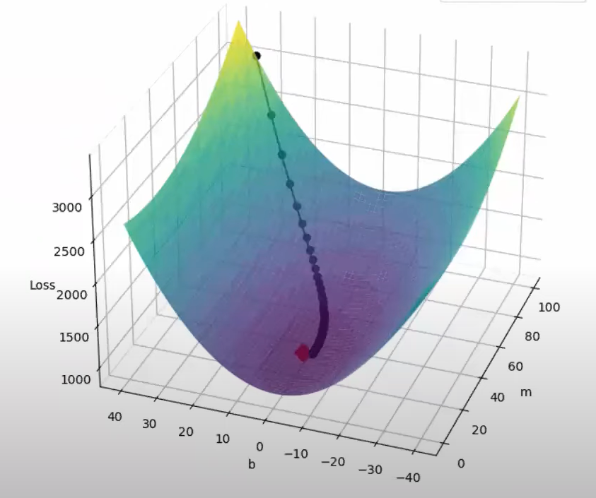
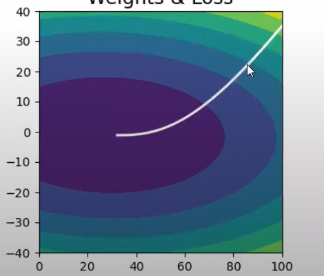
Both batch gradient descent and momentum optimization techniques do not work optimally in case of such data. As depicted in the images , the slope increases quickly in the direction of b(dense data) and then gradually decreases in the  direction of m (sparse data)

As is evident from the images,neither of the optimizers are able to follow a more efficient path ,due to the fixed learning rates.

Batch gradient descent in sparse datasets

Momentum optimizers in sparse datasets

Mathematical representation:

We first calculate the accumulated gradient using the formula

$$G_t=G_{t-1}+g_t^2$$$$G_{t-1}:\text{sum of squared gradients up to the previous step}$$$$g_t^2:\text{is the square of the current gradient}$$$$W_{t+1}=W_t-\frac{\eta }{\sqrt{G_t+ϵ}}\cdot g_t$$

1. $\eta$: is the initial learning rate
2. $G_t$: is the accumulated squared gradients
3. $ϵ$: is a small value (usually around ${10}^{-8}$)
4. $g_t$: is the gradient at the current step
5. $\frac{1}{\sqrt{G_t+ϵ}}$ This term helps in adjusting the learning parameters effectively. The parameters which have a large accumulated gradient $G_t$ will have a slower learning rate, and the ones which have a smaller $G_t$ will have a larger learning rate
6. $ϵ$ is a small value placed to prevent the denominator from becoming zero in case $G_t$ is 0.

In order to elaborate the intuition, we can imagine a loss function in a two-dimensional space, where the gradient of the loss function increases very weakly in one direction and very strongly in the other direction.

If we now sum up the gradients along the axis in which the gradients increase weakly, the squared sum of these gradients becomes very small. Here the learning rate will be very high adn the weight update will be high too. For the other axis, where the gradients increase sharply, the exact opposite is true.

Hence, we speed up the updating process along the axis with weak gradients by increasing these gradients along this axis. Similarly, we slow down the updates of the weights along the axis with large gradients.

• In the weak gradient direction → Higher learning rate → Larger updates

• In the strong gradient direction → Lower learning rate → Smaller updates

The disadvantage of AdaGrad is that since it accumulates the squared gradients, the denominator in the update rule keeps increasing as training progresses. As a result, the effective learning rate keeps decreasing and after many iterations, updates become very small. Eventually, the model stops learning, which in many cases may be before reaching the desired global minima and hence cant converge to the desired solution. However, this problem is seen mostly in deep neural network problems only. AdaGrad works efficiently for linear regression models.

RMSProp (Root Mean Square Propagation)

The main disadvantage of AdaGrad optimizer occurs because we consider the values of "all" the past gradients ($g_t^2$ term which keeps increasing).

RMSProp adapts the learning rate by introducing a moving average of the squared gradients. i.e, The accumulated gradient ($G_t$) term is calculated such that more weightage is given to the gradients of the more recent epochs.

This ensures that the updates are properly scaled for each parameters and prevents the learning rate from becoming too small.

Mathematical representation:

The only change we made from the AdaGrad optimizer is in calculating the velocity term. The second equation remains the same.

$$\beta G_t=(1-\beta )G_{t-1}+g_t^2$$$$\beta :\text{momentum coefficient / decay rate (around 0.95)}$$$$W_{t+1}=W_t-\frac{\eta }{\sqrt{G_t+ϵ}}\cdot g_t$$

RMSProp maintains an optimal learning rate by using a decay rate parameter and hence ensures faster convergence to the desired minima. It is one of the most widely used and efficient optimization algorithm with negligible disadvantages.

Adam

Adam stands for Adaptive Moment Estimation. This method was designed to make the optimization process even faster by combining the logics behind SGD with momentum and Adagrad.

Mathematical representation:

Weight update:

$$W_{t+1}=W_t-\frac{\eta }{\sqrt{G_t+ϵ}}\cdot m_t$$

Momentum (First Moment Estimate)

$$m_t={\beta }_1{m}_{t-1}+(1-{\beta }_1)g_t$$$${\beta }_1:\text{around }0.9$$$$\text{derived from SGD with momentum}$$

Exponentially weighted average of the past gradients

Variance (Second Moment Estimate):

$$v_t={\beta }_2{v}_{t-1}+(1-{\beta }_2)g_t^2$$$${\beta }_2:\text{around }0.99$$$$\text{derived from AdaGrad}$$

This term maintains an adaptive learning constant, ensuring that the past gradients have lesser weightage than the current gradients.

Bias Correction:

We require a bias correction because both momentum term and variance are initially zero and are biased towards 0 at during the start of the training

$$m_t^{\prime }=\frac{m_t}{1-{\beta }_1^t}$$$$v_t^{\prime }=\frac{v_t}{1-{\beta }_2^t}$$$$\text{T: epoch number}$$