Neural Networks in Practice

by Lalith, on 5/11/2024

Neural networks have a lot of moving parts, there's a lot of things you need to build in order to train one. I assume you know all that goes into these networks, if not look at this article before proceeding.

This will be a fairly high level overview of the libraries to create and train neural networks (as per my standards), so I won't go in depth about all the tooling which goes into training these networks. But it's fair to say that these libraries make it really straightforward to create and train your own networks.

Now, what are these libraries? There are quite a few. For example there's Theano (now forked and maintained as PyTensor), TensorFlow with the Keras API, PyTorch, FLAX built on top of JAX, and a bunch of other libraries over the years. Wikipedia has a list of all these libraries which you can browse if you're interested.

An introduction to PyTorch

PyTorch is one of the most used libraries by everyone in the industry. It's a fairly large library, and was a bit late to the game getting to full release, but it has cemented itself firmly as a very capable and highly performant framework.

While it definitely isn't used widely in education (that crown goes to TensorFlow), it has a much nicer interface to build and train models, and also contains the most bleeding edge tech for training the largest models. OpenAI switched over to PyTorch a while ago, not to mention Meta created Pytorch before handing it over to the Linux Foundation to be run under the new Pytorch Foundation.

Tensorflow was created by Google in 2015, which seems to be slowly sunsetting in favour of using JAX/FLAX (which has an API similar to PyTorch) likely due to the relatively poor design of TensorFlow and a rewrite for Google to use their TPUs.

Writing code in PyTorch

Now that the short history lesson of PyTorch is over, let's actually begin writing some code. And nearly every project in PyTorch begins with the mantra of

import torch
from torch import nn
import torch.nn.functional as F
from torch.utils.data import DataLoader
from torchvision import datasets
from torchvision.transforms import transforms

Where we first import the actual torch library, nothing of interest here.

Then we import torch.nn which contains all the classes to build our neural network and its loss functions, followed by torch.nn.functional, which provides us a wrapper over a few classes (mainly loss functions) which we don't want to initialize a library over. F is just a popular shorthand everyone uses.

Then we have the utility classes for handling our data. The DataLoader which allows us to easily iterate over over our dataset without having to deal with all the random sampling, memory pinning, parallelism, etc,.

torchvision is a not a fun API to work with, but that's true for most vision datasets in general. Here we are just importing the datasets we'll be using and transforms library to make sure they're in the right format for our network.

Before we define a network

I'm going to go out of order in terms of the actual code you would actually write, but this allows us to do the fun stuff before we tear our hair out trying to get the dataloader working properly (and efficiently).

I'm going to show three examples of neural networks, each increasing in complexity, but all of them are microscopic compared to networks trained in the past 10 years¹.

Before we begin, we need to first figure out what our data will be, and what we want to classify. I'll be using the MNIST database for this, it's a dataset based off of the original NIST datasets, which are no longer available (likely absorbed under Special Database 19). It was created 30 years ago (1994), though the actual transforms from NIST are also not known.

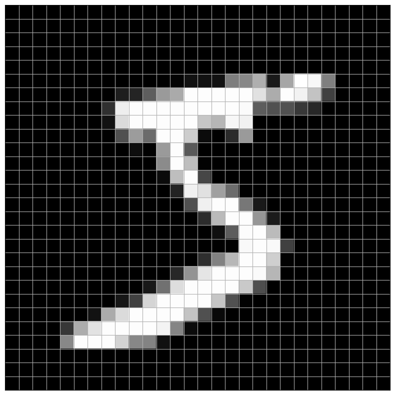
The dataset contains $28 \times 28$ images of digits with only a luminance channel (the original was only bilevel/binary). We'll get back to processing the inputs later, but suffice to say, our inputs will be $784 = 28 \times 28$ numbers representing each pixel in the image.

MNIST_example

Now, our task will be to train a network to predict what digit this is. It's obvious to us that this is probably a 5, but there's no obvious way to write this in code without a lot of effort and a rat's nest of switch cases and if-else statements at the end of it.

The naive approach

Remember that the neural network can only work with numbers which are differentiable, so we can't have the output be a integer as there's no way to differentiate integers².

We could set the model to predict a single number, and round it to the nearest integer and predict that. But there are a few issues with that approach.

What will our loss function be?

We could use a distance metric between the predicted digit and the actual digit, but - for example - the model might learn that 1 and 9 are very distinct or 7 and 8 are very similar and not learn them as the "reward" for spending its "neural capacity" on learning the nuances as the loss function does not reward it.
We could do a binary encoding, where the loss is 0 is the predicted and actual digit are the same, and 1 if they are different. This still won't work as the loss is not differentiable. No worries, we'll just attach a gaussian to the predicted value, now it's differentiable. But we again have the issue of the model learning that 7 and 8 are similar because of the leaky loss, it's better but not ideal.

How much capacity does this consume?

Neural networks have a concept of capacity, where there's only so much information they can contain³. So, we know that these models have a finite capacity, and letting them figure out how to "write" to this number line given the input image is not a trivial task. For example, the Perceptrons book from 1969 gives the famous of example of how a "single layer perceptron" cannot learn XOR. This is obviously not true for multilayer perceptrons⁴ even without activation functions.

So, while it is possible to embed our values and let the model learn it, we're wasting capacity to allow it to learn the structure of the number line.

A better approach

Instead of all of that complicated machinery which we have to invent, we could just have 10 classes each of which predict a single digit. Sure, there are a few disadvantages with this approach compared to the other one. For one, the model has a lot more knobs to tune so that it predicts the right digit. This is not really of much concern though, as we are inducing a bias which we know about the data, where the actual digit shape and it's value are unrelated. In fact, it's better that we think of these digits not as numbers, but as symbols coming from a certain class, so instead of thinking of "4" having the value 4, we think of it as a symbol coming from 10 different classes like cats, dogs, ships, etc,.

We can think of this as a 10-dimensional output space, where we tell the model that each symbol exists purely on one of these axes. But the model can also introduce its own knowledge by keeping covariance the dimension corresponding⁵ to "7" and "1" pretty high as they are digits with similar characteristics⁶.

Defining the network

So, now we know that we want the network to take in 784 values, and return 10 values representing its belief of how much the image corresponds to that symbol. In fact, let's create a network which does just that, nothing fancy in between.

class MyModel(nn.Module):
    def __init__(self):
        super().__init__()
        self.fc1 = nn.Linear(28 * 28, 10)

    def forward(self, x):
        x = x.view(-1, 28 * 28)
        x = self.fc1(x)
        return x

There's a lot to unpack here if you're not familiar with Python, so let's go step-by-step.

Initialization

First, we inherit from nn.Module which is the universal object from which every neural network component is defined from convolutional layers, and even the loss functions.
Then we initialize everything so that torch can hook all our layers into the backprop engine.
Now, here's our first layer we register into our model. It's a linear layer which takes in our 784 neurons and then directly pushes it to 10 classes. This is essentially a matrix of shape $784 \times 10$ with a bias vector of size $10$ .

Forward Pass

Finally, we come over to the forward function. This is a function we're overriding in the base class where we define the forward propagation of our model.
This is probably the hardest part to keep track of, but x.view is the function which does the preprocessing of our image into the right shape. The input to our model is either of shape $(b a t c h_s i z e \times 1 \times 28 \times 28)$ or $(b a t c h_s i z e \times 28 \times 28)$ depending on whether we drop the channels dimension or not.
Obviously, this is not compatible with our input layer which expects something with a final dimension of 784, but we would have 28 in both cases. So, x.view(-1, 28*28) gives us a "view" of our input⁷ of two dimensions, where the final dimension is guaranteed to be 784, with the first dimension being automatically determined. In this case, our output should be of shape $(b a t c h_s i z e \times 784)$ .
self.fc1(x) internally does $W^{T} x + b$ , where $W$ and $b$ are the internal parameters of our linear layer.

Loading the data

We finally come to the part where we can actually turn all of this theory into a tangible model which we can measure. Here's the thing, we still haven't created our model, we've only defined how it should be built and forwarded.

We can create the model by running

model = MyModel()

Now, we have our model, but this model is pointless, it hasn't been trained, we don't even have the data to do it yet.

Let's fix that. First, we need to load our data. Thankfully - if you remember from before - we imported a bunch of libraries from torchvision, which we'll now use.

batch_size = 32

transform = transforms.Compose([
    transforms.ToTensor(),
    transforms.Normalize((0.5, ), (0.5, ))
])

dataset = datasets.MNIST(root="data/", download=True, transform=transform)
dataloader = DataLoader(dataset, batch_size=batch_size, shuffle=True)

The code here is really not illuminating, check the docs if you want more detail, but I'll give a brief overview.

The transform variable here takes the data from MNIST, which we receive as PIL images, so we convert them into torch tensors with ToTensor(), then we normalize the values into the range $[- 1, 1]$ ^8,9.

We then load the data from the datasets module, and apply the transform before feeding it into the dataloader where we make sure the data is shuffled and pass in a batch size for each forward pass.

We can check the data returned by running

X, y = next(iter(dataloader))

print(X.shape) # torch.Size([32, 1, 28, 28])
print(y.shape) # torch.Size([32])

Where the first dimension is always the batch size, followed by the shape of the tensors. We see that the channel is still preserved in our data, but we don't have to worry about that as our model automatically handles that. torch.Size is just a utility class to specify tensor shapes¹⁰.

Building a training loop

Everything is in place for us to train our model now. All that's left is to choose a loss function, attach an optimizer and create the training loop.

We'll be using the Adam optimizer and categorical cross entropy as our loss function.

optim = torch.optim.Adam(model.parameters(), lr=1e-3)
crit = nn.CrossEntropyLoss()

We're using a learning rate of $0.001$ here. And we're passing the model.parameters() generator to Adam, which registers each of the trainable parameters into the backprop graph so torch can keep properly compute the gradients to each of the parameters.

Onto the training loop.

losses = []

def train(epochs):
    for epoch in range(epochs):
        for i, (images, labels) in enumerate(dataloader):
            out = model(images)
            loss = crit(out, labels)
            loss.backward()
            optim.step()
            optim.zero_grad()

            if i % 100 == 0:
                losses.append(loss.item())

        print(f"Epoch: {epoch}, Loss: {loss.item()}")

The training loop consists of us going through our entire dataset epochs number of times, which is the technical term for a single full pass through your training dataset. It is completely unrelated to its use in chronology.

We then forward pass our images through our model using model(images), this internally calls model.forward, but there are hooks which might be missed if we do so manually, but it won't affect anything here. In general, it's a good idea to do model(X) instead of model.forward(X) as it's less code to write in the first place, and we can let torch do whatever optimizations or hooks it needs to internally.

Then we apply our criterion crit on the models outputs and the actual class labels. The full equation of what the criterion does is pretty gnarly, so I'll give you the actual equation which we use instead.

\sum_{i = 0}^{B} \sum_{c \in C} - (y_{i} = c) \log (softmax ({\hat{y}}_{i, c}))

Where $y_{i}$ are the ground truth labels with $i$ being the index over the batch. ${\hat{y}}_{i}$ are the model's "logits", which are non-normalized probabilties the model predicts. We pass this through a softmax to give us probabilties instead of letting the model learn it and wasting capacity. The set $C$ comprises of the symbols ${0, 1, 2, . . ., 9}$ .

For every class, if our label matches the class ( $y_{i} = c$ ), we take the softmax of our logits and add the negative log probabilities of the model predictions as the loss.

The loss is minimized when the softmax is close to 1 as we are taking $- l o g (x)$ and the domain is $[0, 1]$ . The softmax has the property of returning 1 when it's input is the maximum, and near 0 when it's not.

These three lines carry a lot of complexity behind them beyond the scope of this article

out = model(images)
loss = crit(out, labels)
loss.backward() 
optim.step()
optim.zero_grad()

if i % 100 == 0:
    losses.append(loss.item())

loss.backward() writes to the gradient fields of all the parameters. optim.step() uses the gradient to update the weights. optim.zero_grad() zeros out all the gradients for the next training step. The way they perform each of these warrant an article of their own about the internal workings of torch and autodifferentiation engines.

We then keep track of the losses over time and print out the loss every epoch, some basic metrics which you can extend.

Here's some sample output as our model trains (this will be different due to random sampling as we're not pinning our random seed)

train(epochs=6) # or just train(6)

Epoch: 0, Loss: 0.347740113735199
Epoch: 1, Loss: 0.20032547414302826
Epoch: 2, Loss: 0.17316730320453644
Epoch: 3, Loss: 0.12098579108715057
Epoch: 4, Loss: 0.147182434797287
Epoch: 5, Loss: 0.09096773713827133

If we plot the losses which we saved, we get 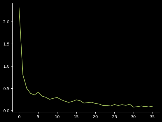losses

The plotting code is pretty simple¹¹, it's just

import matplotlib.pyplot as plt

plt.plot(losses)

We can see that the model is learning a lot at the start, but peters off near the end, this is expected as the inital weights are completely random. But just because they seem to flatten out, doesn't mean there isn't meaningful training going on. If we look at the log of the losses¹²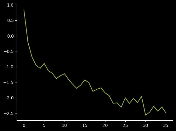 Log losses We can see that it still is learning. Depending on how long you train, your model could achieve state-of-the-art performance if you let it keep training long after it seems to flatten out.

Creating predictions

Now that our model is trained, let's see how it performs when we ask it to predict the labels now.

We can do this by passing images like usual in the forward pass to the model. But instead of just passing its output to nn.CrossEntropyLoss(), we can just take the argmax, this will contain the index the model thinks is the most likely to be the answer.

image, label = dataset.data[1234], dataset.targets[1234]

# index to zero as output is of shape (1, 10, ), so we get (10, )
out = model(image)[0]
predicted = out.argmax().item()

print(f"Model predicts {predicted}, Actual value is {label.item()}")

Here's a sample of model predictions 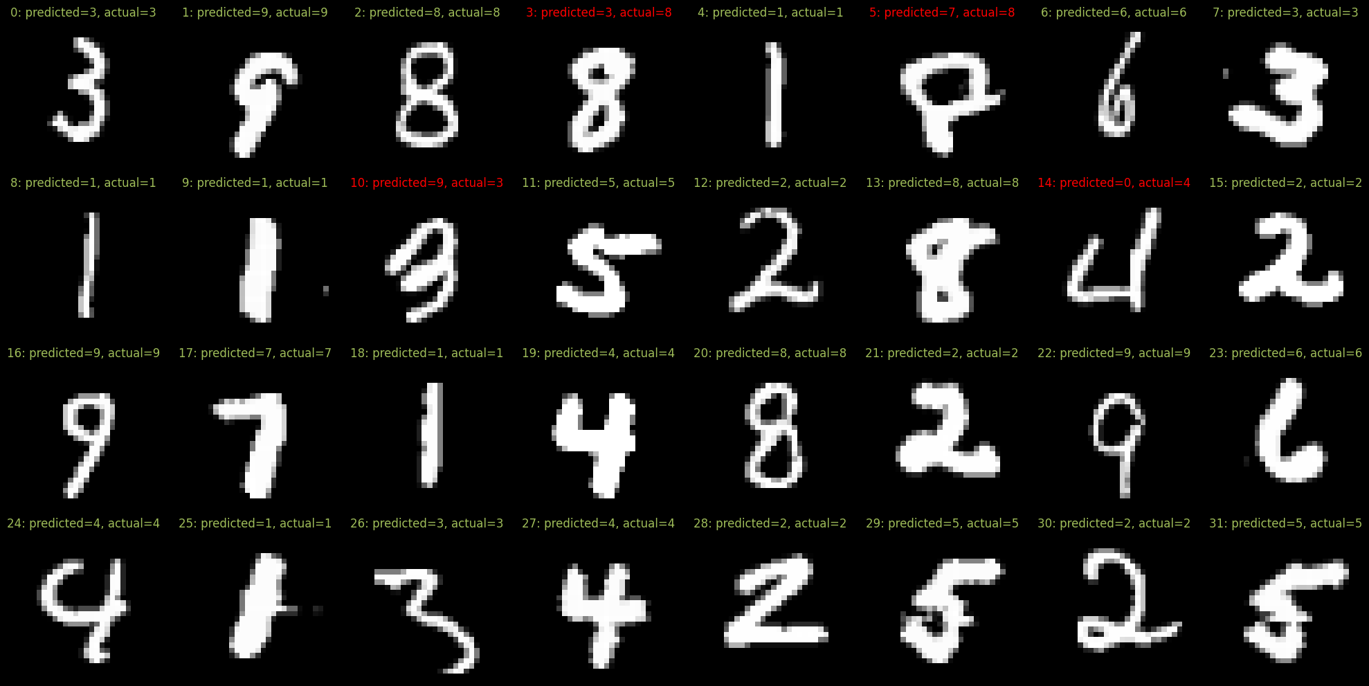prediction samples

As you can see, the model is pretty accurate, but there are some understandable mistakes, but also bizzare ones like it predicting 4 as 0, which should tell you that the model hasn't learnt to recognize the digits in the same way we humans do.

Let's visualize the probabilities of that class. 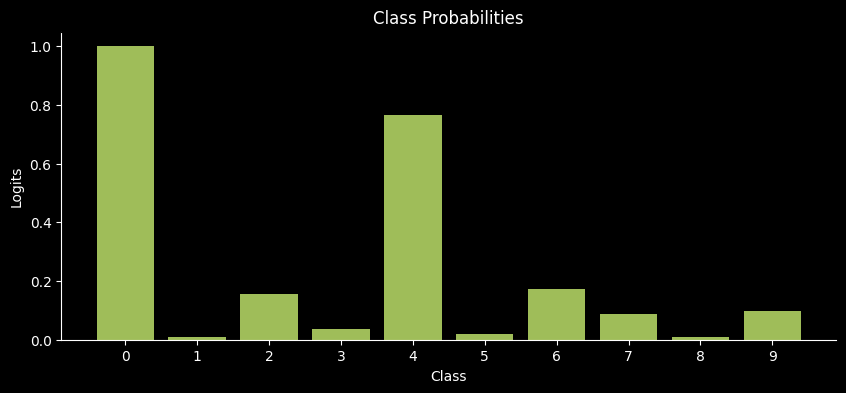probabilties

As you can see, the model is also confident about it being 4, but it's a lot more confident of it being 0.¹³

Other model architectures

Now that we've gone through the entire process of training the model, let's just go through a few other architectures of models for MNIST.

A deeper network

The network we've trained thus far is not really deep. In fact, it's shallower than a run-of-the-mill decision tree¹⁴. Here's a link to a scaled down version of our model to demonstrate how flat it really is. So let's create a deeper network.

class DeeperModel(nn.Module):
    def __init__(self):
        super().__init__()
        self.stack = nn.Sequential(
            nn.Linear(28 * 28, 512),
            nn.ReLU(),
            nn.Linear(512, 512),
            nn.ReLU(),
            nn.Linear(512, 10),
        )

    def forward(self, x):
        x = x.view(-1, 28 * 28)
        x = self.stack(x)
        return x

Here's a pretty standard network architecture for MNIST which you find everywhere. And a scaled down version of the actual model from top to bottom¹⁹. 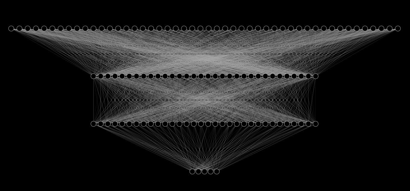Deep network

Each of the lines represent a parameter the model can learn. In this image there are 2720 edges shown, and there are 69¹⁵ biases. For a total of 2789 trainable parameters. The actual network we defined has 240x that at nearly 670k parameters. And this model isn't even large, LLMs easily reach the billions of parameters, and a few even breach trillions of parameters.

For a sense of scale, take the scaling from this image to our actual model. Apply that to our actual model. This now represents your average sized model from 10 years ago. Now scale that model again, now we've finally reached the size of LLaMa-40B, a modestly sized current day model. We haven't quite reached another level of scaling from there yet¹⁶

Okay, enough nerding out about scale. There's a few new parameters I've added here. Let's first look at ReLU.

ReLU here is just a regular class which again inherits from nn.Module, and can be used like any other module, there's really not much of interest here, look at the article about it to learn more.

Then we have nn.Sequential, it's a convenience class which takes an arbitrary number of parameters and registers all of them to be forwarded in the order they were passed in. It's similar to the keras.Sequential if you're familiar with that.

The rest of the snippet is pretty much the same, so there's not much to say here.

Convolutional networks

I'll just brief what convolutional networks are, if you want to learn more look here. We'll build a network very loosely inspired by AlexNet.

class CNNModel(nn.Module):
    def __init__(self):
        super().__init__()
        self.stack = nn.Sequential(
            nn.Conv2d(1, 32, kernel_size=3, stride=1, padding=1),
            nn.ReLU(),
            nn.Conv2d(32, 64, kernel_size=2, stride=2, padding=2),
            nn.ReLU(),
            nn.Conv2d(64, 64, kernel_size=2, stride=1, padding=1),
            nn.ReLU(),
            nn.MaxPool2d(2),
            nn.Flatten(),
            nn.Linear(4096, 1024),
            nn.ReLU(),
            nn.Linear(1024, 10),
        )

    def forward(self, xb):
        out = self.stack(xb)
        return out

This is the largest of all our model at 4.2M parameters. But even this model is miniscule compared to the 2012 AlexNet. I will skim through the overall architecture as it's all covered in the CNN article.

But I'll just detail the parameters as the PyTorch docs are really terse. So, starting off with nn.Conv2d

`nn.Conv2d`

nn.Conv2d(32, 64, kernel_size=2, stride=2, padding=2),
#          1   2              3         4          5

in_channels: This is the number of channels the input image has, in our sequential example it just leads to a bunch of redundant code, but it's pretty useful to define more bespoke architectures.
out_channels: This is the channels the output has, but it's not equal to the number of filters contained. The total number of filters is equal to $i n_c h a n n e l s \times o u t_c h a n n e l s$ which makes this layers parameters quadratic in channels for convolutions which maintain depth.
kernel_size: Pretty self-explanatory, this is the size of the kernel which is learnt inside the layer, it is usually an integer, but you can specify non-square kernels by passing tuple, though that's rarely done in practice. These three layers are the main factors determining the parameter count of the model (bias is the other one), while all the other ones can be considered hyperparameters of the network.
stride: Again, self-explanatory, and also support passing a tuple for different strides across dimensions which gets rarely used.
padding: This also is the same as the other two, except it also accepts two string parameters of 'valid' and 'same'. There seems to be no difference between 'valid' and 0 padding, so I'm not sure why it still exists. 'same' padding ensures that the input and output tensors height and width stay the same, it is only valid when stride=1¹⁷.

There are a few other parameters, but they're very rarely used, you can lookup the docs yourself if you want to know more.

`nn.MaxPool2d`

nn.MaxPool2d(2, 2),
#            1  2

kernel_size: The size of the kernel for which the pooling must occur, this is also used for the stride if one is not provided as that covers the majority of use cases.
stride: Rarely used, but worth mentioning as it's similar to nn.Conv2d's API, it serves the same purpose with the same logic.

Similarly, there are other very rarely used arguments which nearly nobody uses which you can check in the docs.

The rest of the architecture has all been covered, it's just a matter of gluing all these parts together.

Before closing off this section, here's a snippet of code you can use to check the number of trainable parameters your model has.

sum(torch.numel(p) for p in model.parameters())

Where numel stands for number of elements. And model.parameters() returns a generator of all the tensors in the model¹⁸.

Train on a GPU

All the examples so far have been running on the CPU, which is not ideal for training neural networks. Neural networks are rife with numerical computations, and especially matrix computations.

CPUs are optimized to have really low latency instead of throughput. Latency here refers to the time difference between asking the CPU to perform an operation, and the time it takes to actually execute that operation. Throughput is the total number of operations performed over time.

Sure, decreasing your latency will automatically increase your throughput as the CPU will finish each operation quicker so that it can continue to do the next operation.

But there's a way you can trade off your latency for throughput. And GPUs do that exact thing. Instead of having die space allocated to ensure that every operation finishes quickly, they go in the opposite direction to make sure that data can only come in a certain minimum batch size before it can be operated on. This allows more die space to be allocated to computing a large batch of a short list of operations really quickly. And a whole host of other engineering outside of the scope of this article to make sure that the cores are always busy crunching numbers.

There are other chips dedicated for that task, but it's unlikely you have access to them, nor the expertise to optimize your model for the device.

What needs to be changed?

Torch makes it really easy to run computation on a GPU, first you need to figure out if you can use a GPU.

device = torch.device(
    "cuda"
    if torch.cuda.is_available()
    else "mps" if torch.backends.mps.is_available() else "cpu"
)

That's all you need, now you have a handle to a device. print the device to see which one you have. It checks if your computer supports CUDA (Compute Unified Device Architecture) - which is Nvidia's catch-all name for their GPU architecture and SDK - else if you have a Mac with mps support, it'll use that, and fall back to CPU if all else are unavailable.

If you want to train your model on the GPU, the only line of code you need to add before the training loop is model.to(device), and you're done.

Well, there'll be a bunch of errors you'll get if you just launch the training loop now though. Because you also need to move all the tensors which were created on your CPU to the GPU. So, changes like images.to(device) and labels.to(device). It's a pretty tedious process, but fairly straightforward.

You probably won't see much GPU usage with our models as they are rather tiny compared to models which actually need to train on GPU. And there's also other bottlenecks related to your dataloader and bandwidth limitations because of the frequent swapping for minibatches. Some of these can be mitigated, but they are out of scope of this article.

To close off, I'll just detail how you can save and load these models so that you can share them. It's just two commands

torch.save(model.state_dict(), "model.pth")

model.load_state_dict(torch.load("model.pth")) # Optionally pass `weights_only=True` to torch.load

Torch saves models by saving the dictionary of the models weights, and loading them by inserting back into that dictionary. This gives you one caveat. You just can't load the entire model without knowing the architecture, so if you have a really complex forward pass, it might be impossible for someone to reconstruct your model from just the weights. Making the weights pointless.

You still need to have the model class, initialize it, and then you can insert the state_dict into it. So, you'll need to ship the code of how the model can perform a forward pass (which usually entails the entire model architecture) for you to deploy your model.

Conclusion

This just a small overview of all the features of PyTorch. We've explored each of the features in-depth, but there's still a lot more which can be covered, especially relating to activation functions, the functional API, other kinds of layers, and the torchvision library.

We'll be continuing to write articles on this, if you have any ideas of articles you want us to write, or any explanations you'd like update, you can reach out to us.

^[1] The largest one I'll be showing is 15x smaller than AlexNet, the first CNN to be successfully trained on a GPU.

^[2] There are, but it's out of scope of this article.

^[3] This is true for any finite set of numbers, if you're interested look into informataion theory and specifically the source coding theorem and rate-distortion theory, it's a pivotal part of data compression and plays a major role in machine learning overall.

^[4] Perceptrons are just a regular dense/linear layer you've heard about, just with a more bespoke name becauase it's from the 60's

^[5] Notice that it doesn't actually need to be the 7th dimension, but I'll call it dimension 7 for brevity

^[6] This idea of the model learning stuff in higher dimensions by learning the covariance, and how the "surface area" for this grows exponentially can be seen with this lemma

^[7] The view doesn't create a new tensor, it creates an indexing schema if the shapes are compatible, otherwise it throws an error. Tensor.reshape does the same thing, but it creates a copy of the tensor if the shapes are not compatible, which might go unnoticed and you may lose training performance due to it.

^[8] Just to detail the actual transform, the values it takes are "mean" and "standard deviation", where you specify them both, but the actual transform it does is just $\frac{X - μ}{σ}$ . The thing is, this does not guarantee that the mean nor std will be the values you specify, so it's just a regular linear transform, and not a "normalization".

^[9] We put it in the range $[- 1, 1]$ because it gives the model the ability to use the structure of being signed (which it can still do with a bias, but again, capacity). This is especially useful in ReLU and its variants as they have a lot of structure associated below 0.

^[10] The reason this exists is mostly an artifact of PyTorch's internals being written in C++, but it's also useful when you want to do something specific with the shape of your tensors on device without having to access memory of different devices. This mostly applies to GPU training, which is not the focus of this tutorial.

^[11] The code to make that color scheme is not, it's just a huge mess considering the legacy codebase that matplotlib is, but the core idea remains the same

^[12] Try recreating this yourself by mapping the losses to log

^[13] You might have noticed that these softmax probabilities don't add up to 1. This is because the actual softmax probabilities would show "0" near 1, while the rest were near 0, to fix this, I added a bias to all the values so that they are closer to each other. This process is exactly the same as increasing the "temperature" of the output layer of LLMs (upto a normalization factor).

^[14] [Insert joke about LLMs being shallow]

^[15] Yes, it's exactly 69_nice , it wasn't even intentional. The first linear layers adds 32 biases, the 2nd also adds 32, and the final one has 5, which sums up to 69.

^[16] The next milestone is at 10T parameters. For context, OpenAI's GPT-4 is approximately 1.8T parameters (though that is using MoE, which means not all the parameters are active at once). If we scale up 5x, we'd have reached another scaling from the "microscopic" model shown.

^[17] Probably because strides $\geq 2$ would automatically require adding more padding than image, there's no technical reason preventing it from being an option, it's one of the rare examples of torch idiot-proofing their API

^[18] The values in the generator are of type torch.nn.parameter.Parameter which is not what torch.numel accepts, but it turns out the interface on Parameter is nearly identical to Tensor, so it just works

^[19] Activation functions omitted, or imagine them to be in the neurons, these diagrams are really just a simplification of the actual model. For example, the one in the diagram can be written as

W_{1}^{T} (R e L U (W_{2}^{T} (R e L U (W_{3}^{T} x + b_{3})) + b_{2})) + b_{1}

but that doesn't really tell you much about the model.

Neural Networks in Practice ​

by Lalith, on 5/11/2024 ​

An introduction to PyTorch ​

Writing code in PyTorch ​

Before we define a network ​

The naive approach ​

What will our loss function be? ​

How much capacity does this consume? ​

A better approach ​

Defining the network ​

Initialization ​

Forward Pass ​

Loading the data ​

Building a training loop ​

Creating predictions ​

Other model architectures ​

A deeper network ​

Convolutional networks ​

nn.Conv2d ​

nn.MaxPool2d ​

Train on a GPU ​

What needs to be changed? ​

Sharing models ​

Conclusion ​